I recently read an article in a well-known consumer-facing technical hobby magazine, where the author used the phrase, “watts per day.” This is an erroneous concept (the technically-trained author should have known better), which illustrates a matter that is often confusing to the average person.
“Watts per day” is not a meaningful unit of measurement.
The watt (W) is a unit of power, which is defined as the rate at which energy is transferred or used. One watt is equal to one joule per second (J/s).
The unit of energy is typically measured in joules (J), but it is also commonly measured in watt-hours (Wh) or kilowatt-hours (kWh). One watt-hour is equal to one watt of power used for one hour, and one kilowatt-hour is equal to one kilowatt (1000 watts) of power used for one hour.
In other words, the “watt” conveys the notion of the rate of energy consumption. When we pay for energy consumed, we pay for kilowatt-hours.
Therefore, if you see the phrase “watts per day,” it is likely that the author was trying to convey the notion of power used over a period of one day, and the correct usage would be to express it in terms of watt-hours (or kilowatt-hours) per day.
As an example: if a piece of equipment is rated at 100 watts, and the equipment is used for 8 hours every day, then we can say that the equipment consumes 800 watt-hours of energy (not power) per day.
The FCC has proposed in an NPRM to impose license fees on Radio Amateurs. I urge you to send your comments to the FCC arguing against the reinstatement of those license fees.
You may not be aware of the public good this service provides in times of emergency, as it has during the recent hurricanes. The decrease of new applicants in recent years is not helped by this mercenary proposal.
You may also not know that amateur radio is often a leading developer of new technologies. Just one example is the recent development of a low-cost vector network analyzer — the NanoVNA. Originally developed by and for radio amateurs, this breakthrough device is now being used in the broadcast and other wireless industries, as written up by broadcast engineer Doug Lung in the last two issues of IEEE BTS Magazine and in TV Technology.
Modulation is the process of imparting a signal, usually audio, video, or data, onto a high-frequency carrier, for the purpose of transmitting that signal over a distance.
Let’s take a carrier signal, cos(ω_c t)and a modulating signal, cos(ω_m t), where ω = 2 \pi f , and f is the signal frequency.
Amplitude modulation is simply the product of the carrier signal and (1 + modulating signal):
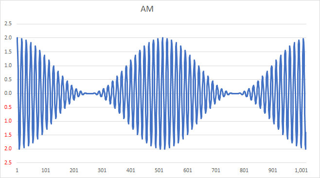
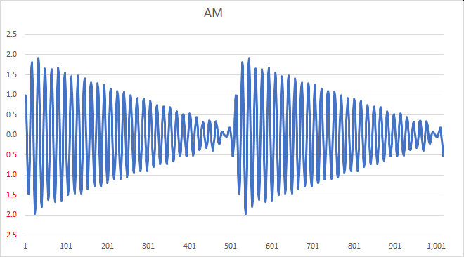
which multiplies out as: AM(t) = cos(ω_c t) + cos(ω_c t)\times cos(ω_m t) ] . A carrier modulated by a sine wave is shown in the following example.
Note that such a signal is relatively easy to demodulate: a simple rectifier and low-pass filter will recover the modulation from this signal, as you can visualize by “erasing” the negative portion of the signal and averaging over the remaining waveform. Such a process is called envelope detection.
To analyze the composition of this signal, we take the trig product identity, cos(x)\,cos(y) = \frac{1}{2} [ cos(x-y)+cos(x+y) ], and apply it to the product term in AM(t), producing the following:
\displaystyle AM(t) = cos(ω_c t) + \frac{1}{2} cos(ω_c t - ω_m t) + \frac{1}{2} cos(ω_c t + ω_m t) .
From this, we observe an important aspect of the process: amplitude modulation results in a signal composed of the following three components:
the carrier signal, cos(ω_c t),
a lower sideband signal, \frac{1}{2} cos(ω_c t - ω_m t),
and an upper sideband signal, \frac{1}{2} cos(ω_c t + ω_m t).
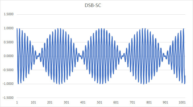
By the way, the reason for the “1 + ” term in the modulation equation above is that it specifically generates the carrier component in the modulated signal. Without it, we would have the following Double-Sideband-Suppressed Carrier signal, which should make it apparent that we can’t use a simple envelope detector to demodulate; note how the envelope “crosses over” itself:
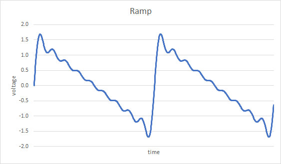
An analysis of modulation is aided by using a more complex modulating signal. A ramp signal is comprised of a fundamental sinusoid and integer harmonics of that fundamental. For illustration purposes, we will take an approximation that uses the fundamental and the next 8 harmonics. This modulating signal is shown below, as a function of time.
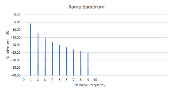
The spectrum of this signal, i.e., a plot of the frequency components versus level, is shown next; it consists of a fundamental (at “1”), followed by a series of harmonics with decreasing levels.
If we amplitude modulate a carrier with this ramp signal, we get the following time-varying signal; note again that this signal can be demodulated by an envelope detector:
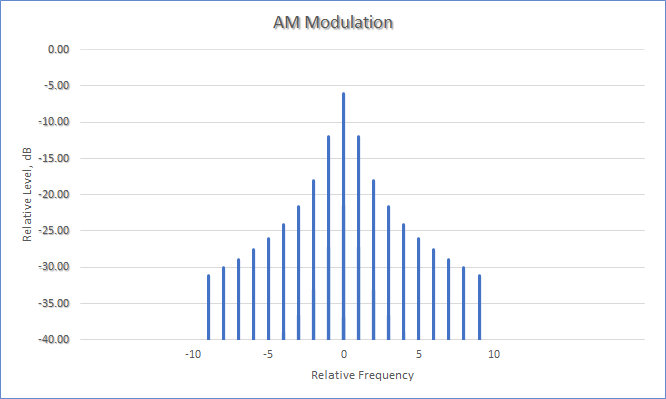
The spectrum of the modulated ramp signal follows; note that there is a carrier at “0” and sidebands extending in both the positive and negative frequency directions. (In practice, this zero point would actually be at some high frequency, such as at 7 MHz for example. The spacing of the individual components in this example would be exactly that of the frequency of the fundamental component of the ramp signal.)
Recall from our earlier discussion that amplitude modulation results in a signal composed of the three components, the carrier signal, a lower sideband signal, and an upper sideband signal. Note the following as well: because the lower sideband component has a negative modulating-frequency term (cos(ω_c t - ω_m t), for a sine wave) the spectrum of the lower sideband is reversed compared with that of the upper sideband (and that of the baseband modulating signal).
We can also see from this example that amplitude modulation is rather wasteful of spectrum space, if our goal is to take up as little bandwidth as possible. For one, the two sidebands are merely reflections of each other, i.e., each one carries the same information content. For another, the carrier itself is unnecessary for the communication of the modulating signal as well — something that wastes power on the transmission side.
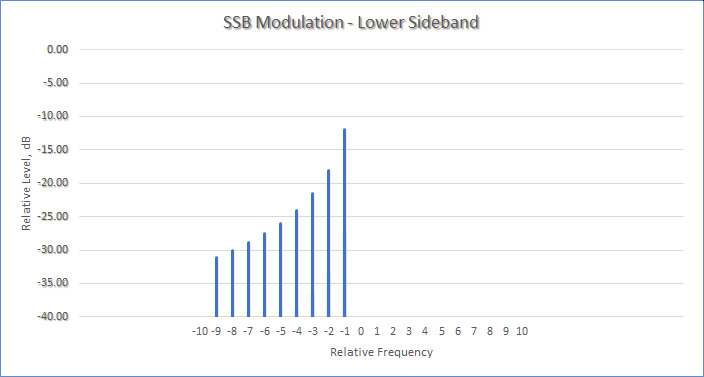
Taking that into account, we can choose to transmit only one sideband, resulting in a Single Sideband (SSB) Transmission. If we transmit only the lower sideband, its spectrum will look like this (note that the carrier is also absent):
SSB modulation can be implemented using a variety of methods, including an analog filter, or phase-shift network (PSN) quadrature modulation. (For a clue as to how PSN works, look up and calculate the result of adding cos(x) cos(y) + sin(x) sin(y).)
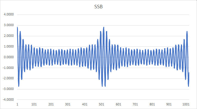
The challenge in receiving this signal is how to demodulate it, as we can see from its time-domain plot:
As compared with amplitude modulation, a SSB signal cannot be demodulated with an envelope detector, because the envelope is no longer a faithful representation of the original signal. One way to demodulate it is to frequency-shift the signal down to its original range of baseband frequencies, by using a product detector which mixes it with the output of a beat frequency oscillator (BFO).
One can appreciate that, if the demodulator BFO is not exactly at the original carrier frequency, the resulting demodulated signal will be frequency-shifted up or down by the amount of the error, resulting in a kind of “Donald Duck”-sounding voice signal. While this was often an issue with analog transmitters and receivers, whose carrier frequencies were imprecise, and would drift over time, modern digital equipment is so accurate that a near-perfect re-synchronization is not difficult to achieve.
The advent of low-cost antenna analyzers and vector network analyzers (VNAs) has resulted in a renewed interest in an 80-year old tool called the Smith chart, a graphical device used to view the characteristics of RF transmission lines, antennas, and matching circuits, and to aid in the design of those systems. But although questions regarding the chart appear in the Amateur Extra License exam, the current Question Pool has a mere 11 questions on the topic, leaving a full appreciation of the tool to the more inquisitive student. Here then, is a brief introduction to the Smith chart.
Motivation
Why use a seemingly-archaic tool such as the Smith chart, when calculators and software are readily available? For one, the chart remains useful as a visualization tool, representing a wealth of information in a very precise and intuitive manner. In addition, the knowledge gained in its use adds to our general knowledge of radio systems. And that’s what ham radio’s all about, right? Otherwise, we may as well use a telephone or the Internet to communicate over large distances! And don’t worry; we’ll keep the equations to a minimum (or in footnotes).
Phillip Smith, 1ANB (SK), was an electrical engineer who graduated from Tufts College in 1928, and then went to work in the radio research department at Bell Telephone Laboratories. Fascinated by the repetitive nature of the impedance variation along a transmission line and its relation to the standing-wave amplitude ratio and wave position, Smith devised an impedance chart in which standing-wave ratios were represented by circles. In 1939, he had an article published in Electronics Magazine describing what later came to be known as the Smith chart.
Derivation
The Smith chart provides a concise way to view a number of different characteristics of RF systems, such as impedance and voltage standing-wave ratio (VSWR). We’ll use an example to show how the Smith chart was developed.
Radio operators are inherently familiar with the concept of standing-wave ratio, i.e., a measure of how well a load is matched to a transmission line. A slightly more obscure concept is that of the reflection coefficient. Notated using the Greek letter gamma (Γ), the reflection coefficient describes how much of an electromagnetic wave is reflected by an impedance discontinuity such as a mismatched load. (For a perfect termination, Γ=0, an open termination yields G=1, and a short results in Γ=-1.) Being a complex quantity, Γ can convey both the magnitude and phase of the reflected wave, at a particular frequency.[1], [2]
We can measure Γ by connecting a VNA to a device under test (DUT), “sweep” a band of interest, and download the data. Our DUT for this example is a 50-ohm coaxial transmission line terminated by a 40m OCF dipole.
First, let’s plot the real and imaginary components of Γ for this DUT on a rectilinear graph. See Figure 1: the green marker is at 14.175 MHz.
Reading off the chart, we see the following values:
frequency
14.000 MHz
14.175 MHz
14.350 MHz
Γ
-0.12 + j 0.26
0.05 + j 0.20
0.08 + j 0.07
Because complex numbers can also be represented in polar form, we can also plot Γ on a polar plot, as in Figure 2. On this plot, the same green marker is now at a magnitude (denoted as |Γ|) of about 0.2 (i.e., its distance from the center or origin), and a phase angle of about 75°. (Note that the curve did not change shape, only the axes of the graph did.) It’s useful to note that the magnitude of the reflection coefficient can never exceed 1.0, as this would imply that power is somehow “created” by the load. This means that Γ is constrained to be within this circular space, such that |Γ|≤ 1.
Smith was no doubt very familiar with the polar type of data presentation, for a practical reason. Back in the day, it would have been rather difficult to measure Γ directly as a complex quantity, due to the limitations of test equipment. But it would have been much easier to measure the polar representation: what was required was an oscilloscope and directional couplers. With these, one could measure the magnitude and phase angle of a wave reflected from a termination, and plot them on a polar graph of the complex reflection coefficient. A simple trigonometric transformation converts these to the rectangular format.[1]
There are several quantities that can be derived from the reflection coefficient. For one, the VSWR is easily calculated from the magnitude of Γ, and is shown in Figure 3.[2]
Figure 3. VSWR of DUT.
Another is the complex impedance, which is also easily calculated from the reflection coefficient at that same “reference plane,” i.e., the point at which the measurement is taken. Because this transformation is so elegant (and important), we present it here:
[1] Because RF components behave differently at different frequencies, engineers use complex numbers to describe impedances and related concepts. The impedance measured at the input to an antenna, at a particular frequency, is expressed as a complex number in the form Z = R + jX, where R represents the real value of the impedance (in ohms), X represents the imaginary value (also in ohms), and j is the imaginary constant \sqrt{-1}.
[2] The quantity Γ is also denoted by the scattering parameter s11. S-parameters generally describe the input-output relationship of RF networks; another such s-parameter is s21, which represents the power transferred to a “Port 2” from a “Port 1” of a network.
In other words, knowing the reflection coefficient Γ and the characteristic impedance Z0 of a transmission line connected to a load, we can directly calculate the load impedance ZL.[3] (As we know, in radio engineering, Z0 is usually 50Ω; video plants commonly use 75Ω, and telephone networks use 600Ω.)
Applying this transformation to our example data, we can produce a graph of the complex load impedance, as in Figure 4, with some interesting observations. First, although the curve looks similar to that of the reflection coefficient, the shape cannot be the same for the following reason: as we learned before, while the reflection coefficient is bounded to a magnitude of 1, the impedance can take on values from zero to infinity. Indeed, if Γ is close to 1, the load impedance can be very high, usually on the order of thousands of ohms.
Figure 4. Normalized Complex Impedance of DUT.
The other useful observation is that, while Γ can have both positive and negative real and imaginary components, the real (resistive) part of the complex impedance can only be positive,[4] and can range from 0 to +∞, while the imaginary part can range anywhere from −∞ to +∞.
From a practical standpoint, this means that conventional (linear) representations of both reflection coefficient and impedance suffer from a number of shortcomings: impedance plots that cover a large extent (e.g., traversing a region close to Γ = 1) would be unwieldy and lack precision; simultaneous plots of different systems would be hard (or impossible) to compare; multiple graphs would be needed to convey information that is intrinsically related; and the conventional representations would be limited to some applications of analysis, while impeding the practicality of system design.
[1] If we denote the phase of Γ by θ, then \Gamma=\left |\Gamma \right |\cdot (\cos \theta +j\cdot \sin \theta) .
[3] Keep in mind that ZL and Γ are complex quantities, so complex arithmetic must be used!
[4]There is no such thing as negative resistance (!), except in tunnel diodes, but that’s another story.
The Smith chart
Phillip Smith understood these limitations, and set forth to overcome them. He brilliantly realized that the various concepts of impedance, reflection, and VSWR could become graphically interrelated by means of the right coordinate transformation – and this would solve the “infinite extent” problem, as well.
Smith’s insight was to start with a rectangular grid of complex impedance, and then warp the axes according to the transformation given in Equation 1. This has the effect of throwing away the negative real (resistance) part, and wrapping the imaginary (reactance) axis so that the points at −∞ and +∞ meet each other. Thus was born his eponymous chart, shown in Figure 5.
The chart consists of a number of internally-tangent circles, and arcs of circles; the number of circles and arcs is simply a function of the desired precision, and charts can also be constructed that “zoom-in” on a particular region of interest. Looking first at the circles, we see they are all internally tangent at a point on the right-hand-side, as seen in Figure 6. Each of these circles represents a constant real (resistive) component, with the circles ranging from 0 ohms (as indicated at the extreme left of the horizontal line – the real, or resistance, axis) to +∞ ohms (as indicated at the extreme right of the horizontal line).
Figure 6. Resistance circles on Smith chart.
Intersecting these circles are arcs of circles that have centers lying on a line (not shown) that is perpendicular to the horizontal line, and which all pass through the point at +∞ ohms. (See Figure 7.) Each of these arcs represents a constant imaginary (reactive) component. The outermost full circle is the imaginary, or reactance, axis.
Figure 7. Reactance circles on Smith chart.
A few definitions and we’re there. You’ll recall from Equation 1 that the load impedance ZL can be calculated by knowing Γ and the characteristic impedance Z0. We can rewrite this equation in a form that normalizes the impedances by dividing both sides of the equation by Z0, which produces Equation 2:
With this normalization, we can use the Smith chart for any characteristic impedance, as long as we remember that the point at the center represents that characteristic impedance. Inspecting the chart, and from the above definitions, we see that the point at the chart center has a value of 1 + j·0, i.e., 1.
The last component to observe is the outermost scale, which is calibrated in degrees and fractions of a wavelength. Among the useful properties of the Smith chart is the fact that adding a length of transmission line has the effect of rotating the complex reflection coefficient clockwise around the chart center, by an angular amount that is proportional to the added electrical length divided by the operating wavelength.
For example, if we add 4 meters of RG-8X transmission line (with velocity factor 0.82) to a system operating at a wavelength of 21.2 meters, the curve will rotate[1] by the following angle:
[1] One wavelength corresponds to two complete rotations around the Smith Chart, hence the 720° factor. Note that adding multiples of ½ wavelength simply brings us back to the same point!
Returning to our DUT, we can now appreciate the utility of this marvelous tool. Using the data from Figure 1, if we now take the reflection coefficient curve of our system, and “drop” it onto the Smith chart (see Figure 8), we can read off the following normalized impedance information (and calculate the actual impedance, shown on the table’s third line, by multiplying by Z0 = 50Ω): [1], [2]
Figure 8. Reflection Coefficient plotted on Smith chart. Green marker is at 14.175 MHz.
14.000 MHz
14.175 MHz
14.350 MHz
ZL/Z0
0.68 + j 0.38
1.02 + j 0.41
1.16 + j 0.15
phase(Γ)
116°
76°
38°
ZL , Ω
34 + j 19
51 + j 20.5
58 + j 7.5
[1] It’s important to realize that the scales on the chart are actually performing the calculation for us; we started with a curve of Γ on a conventional polar graph, and copied that same curve onto the Smith chart, where it now represents Z. It’s only the axes that have changed.
[2] To get the phase of a point, draw line from the center through the point, and extend it to the outer scales, where you can read it off the 0-180° scale.
You may have noticed that the VSWR formula given previously looks curiously similar to the normalized impedance formula given at Equation 2, which leads to another wonderful property of the Smith chart: if you take any point on an impedance plot, and rotate it, around the center, to land on the right-hand half of the resistance axis, the value at that axis is the VSWR at that frequency! (See magnified center at Figure 9.) Note how rotating the green dot would intersect the horizontal axis at the value 1.5, which is what we calculated earlier. In fact, any point on the red circle has a VSWR of that same value. So, when analyzing (or designing) a system with a target VSWR, make sure that the normalized impedance values over the entire frequency of interest remain inside such a circle.
Figure 9. Magnified center of Smith chart; red circle indicates VSWR=1.5.
We specifically chose a limited range of frequencies to keep the visuals simple; in practice, extending the frequency over a wider range leads to some very interesting results! Note too, that while many of these measurements were originally done using paper-and-pencil (and drafting tools), we can easily do the equivalent by using graphical software that directly interfaces to a modern VNA.
Further Reading
Unfortunately, Smith’s own treatise, Electronic Applications of the Smith Chart in Waveguide Circuit and Component Analysis, published in hardcover in 1969, has been out of print for several years, and used copies fetch a premium price. Readers interested in an in-depth elaboration of the chart, as well as examples of using the chart to design transmission elements like matching networks, are directed to the ARRL Handbook Supplemental Articles and The ARRL Antenna Book. Many online resources are available as well, including an Oral History of Phillip Smith, and the Wikipedia page, Smith Chart.
Afterword
As of this writing, the Smith Chart on the Wikipedia page has a small typo; can you find it?
The author has an original copy of Smith’s book, complete with intact transparent overlays — one of his cherished antiques.
Prior to his DTV work, Aldo developed various audio, content delivery and broadcast technologies at CBS Laboratories. He was also Chief Engineer at WKCR-FM and a broadcast engineer at WABC and WPLJ, all in New York City.
A speaker at various industry conferences, he is the author of numerous technical papers and industry reports, including chapters in the 10th and 11th editions of the NAB Engineering Handbook, and has been a regular contributor to several trade publications.
Aldo Cugnini has worked with and studied under several widely-respected authorities in their fields. He has benefited greatly from having known them and others:


 Aldo holds