Modulation is the process of imparting a signal, usually audio, video, or data, onto a high-frequency carrier, for the purpose of transmitting that signal over a distance.
Let’s take a carrier signal, cos(ω_c t) and a modulating signal, cos(ω_m t), where ω = 2 \pi f , and f is the signal frequency.
Amplitude modulation is simply the product of the carrier signal and (1 + modulating signal):
\displaystyle AM(t) = cos(ω_c t) \times [1 + cos(ω_m t)] ,
which multiplies out as: AM(t) = cos(ω_c t) + cos(ω_c t)\times cos(ω_m t) ] . A carrier modulated by a sine wave is shown in the following example.
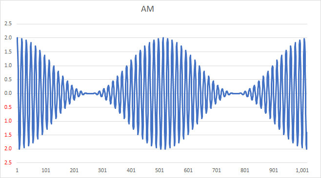
Note that such a signal is relatively easy to demodulate: a simple rectifier and low-pass filter will recover the modulation from this signal, as you can visualize by “erasing” the negative portion of the signal and averaging over the remaining waveform. Such a process is called envelope detection.
To analyze the composition of this signal, we take the trig product identity, cos(x)\,cos(y) = \frac{1}{2} [ cos(x-y)+cos(x+y) ], and apply it to the product term in AM(t), producing the following:
\displaystyle AM(t) = cos(ω_c t) + \frac{1}{2} cos(ω_c t - ω_m t) + \frac{1}{2} cos(ω_c t + ω_m t) .
From this, we observe an important aspect of the process: amplitude modulation results in a signal composed of the following three components:
-
- the carrier signal, cos(ω_c t),
- a lower sideband signal, \frac{1}{2} cos(ω_c t - ω_m t),
- and an upper sideband signal, \frac{1}{2} cos(ω_c t + ω_m t).
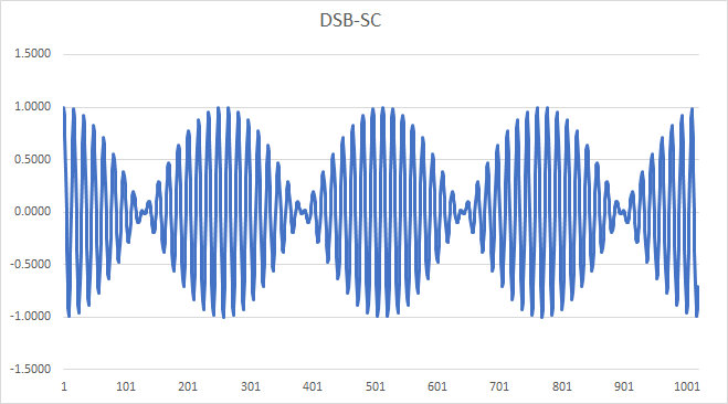
By the way, the reason for the “1 + ” term in the modulation equation above is that it specifically generates the carrier component in the modulated signal. Without it, we would have the following Double-Sideband-Suppressed Carrier signal, which should make it apparent that we can’t use a simple envelope detector to demodulate; note how the envelope “crosses over” itself:
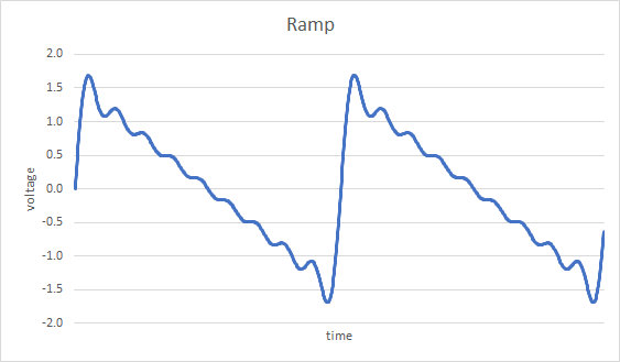
An analysis of modulation is aided by using a more complex modulating signal. A ramp signal is comprised of a fundamental sinusoid and integer harmonics of that fundamental. For illustration purposes, we will take an approximation that uses the fundamental and the next 8 harmonics. This modulating signal is shown below, as a function of time.
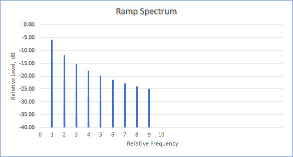
The spectrum of this signal, i.e., a plot of the frequency components versus level, is shown next; it consists of a fundamental (at “1”), followed by a series of harmonics with decreasing levels.
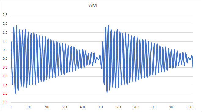
If we amplitude modulate a carrier with this ramp signal, we get the following time-varying signal; note again that this signal can be demodulated by an envelope detector:
The spectrum of the modulated ramp signal follows; note that there is a carrier at “0” and sidebands extending in both the positive and negative frequency directions. (In practice, this zero point would actually be at some high frequency, such as at 7 MHz for example. The spacing of the individual components in this example would be exactly that of the frequency of the fundamental component of the ramp signal.)
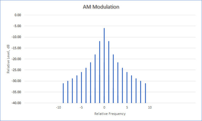
Recall from our earlier discussion that amplitude modulation results in a signal composed of the three components, the carrier signal, a lower sideband signal, and an upper sideband signal. Note the following as well: because the lower sideband component has a negative modulating-frequency term (cos(ω_c t - ω_m t), for a sine wave) the spectrum of the lower sideband is reversed compared with that of the upper sideband (and that of the baseband modulating signal).
We can also see from this example that amplitude modulation is rather wasteful of spectrum space, if our goal is to take up as little bandwidth as possible. For one, the two sidebands are merely reflections of each other, i.e., each one carries the same information content. For another, the carrier itself is unnecessary for the communication of the modulating signal as well — something that wastes power on the transmission side.
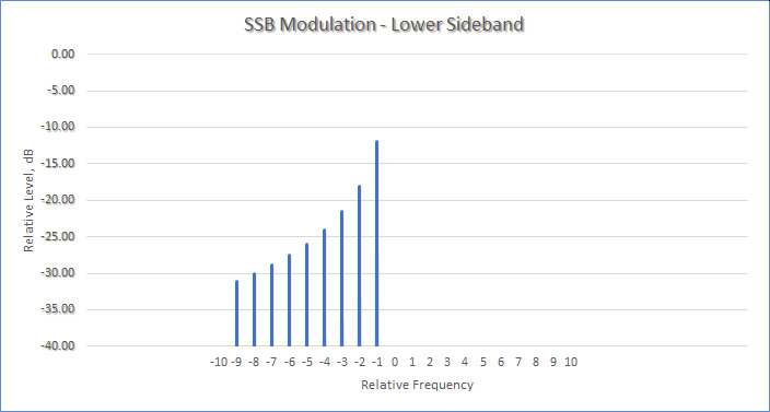
Taking that into account, we can choose to transmit only one sideband, resulting in a Single Sideband (SSB) Transmission. If we transmit only the lower sideband, its spectrum will look like this (note that the carrier is also absent):
SSB modulation can be implemented using a variety of methods, including an analog filter, or phase-shift network (PSN) quadrature modulation. (For a clue as to how PSN works, look up and calculate the result of adding cos(x) cos(y) + sin(x) sin(y).)
The challenge in receiving this signal is how to demodulate it, as we can see from its time-domain plot:
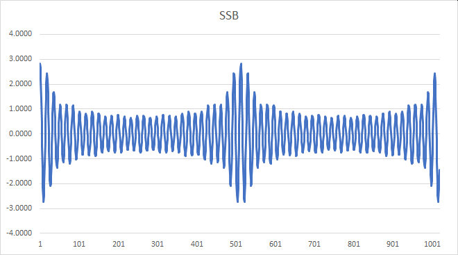
As compared with amplitude modulation, a SSB signal cannot be demodulated with an envelope detector, because the envelope is no longer a faithful representation of the original signal. One way to demodulate it is to frequency-shift the signal down to its original range of baseband frequencies, by using a product detector which mixes it with the output of a beat frequency oscillator (BFO).
One can appreciate that, if the demodulator BFO is not exactly at the original carrier frequency, the resulting demodulated signal will be frequency-shifted up or down by the amount of the error, resulting in a kind of “Donald Duck”-sounding voice signal. While this was often an issue with analog transmitters and receivers, whose carrier frequencies were imprecise, and would drift over time, modern digital equipment is so accurate that a near-perfect re-synchronization is not difficult to achieve.
— agc
/ / /